REGRESSION USING THE DATA ANALYSIS ADD-IN
This requires the Data Analysis Add-in: see Excel 2007: Access and Activating the
Data Analysis Add-in
The data used are in carsdata.xls
The method is explained in Excel
2007: Two-Variable Regression using Data Analysis Add-in
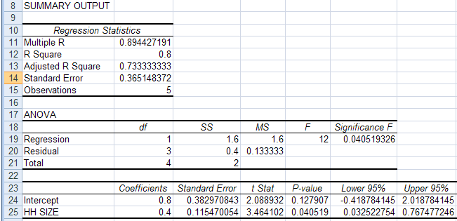
Regression of CARS on HH SIZE led to the following Excel output:

The regression output has three components:
INTERPRET REGRESSION STATISTICS TABLE
| Explanation | ||
| Multiple R | 0.894427 | R = square root of R2 |
| R Square | 0.8 | R2 = coefficient of determination |
| Adjusted R Square | 0.733333 | Adjusted R2 used if more than one x variable |
| Standard Error | 0.365148 | This is the sample estimate of the standard deviation of the error u |
| Observations | 5 | Number of observations used in the regression (n) |
The Regression Statistics Table gives the overall goodness-of-fit
measures:
R2 = 0.8
Correlation between y and x is 0.8944
(when squared gives correlation squared = 0.8 = R2 ).
Adjusted R2 is
discussed later under multiple regression.
The standard error here refers to the estimated standard deviation
of
the error term u.
It is sometimes called the standard error of the regression. It equals
sqrt(SSE/(n-k)).
It is not to be confused with the standard error of y itself (from
descriptive statistics) or with the standard errors of the regression
coefficients
given below.
INTERPRET ANOVA TABLE
| df | SS | MS | F | Signifiance F | |
| Regression | 1 | 1.6 | 1.6 | 12 | 0.04519 |
| Residual | 3 | 0.4 | 0.133333 | ||
| Total | 4 | 2.0 |
The ANOVA (analysis of variance) table splits the sum of squares into its components.
Total sums of squares
= Residual (or error) sum of squares + Regression (or explained) sum
of squares.
Thus Σ
i (yi - ybar)2 = Σ
i (yi - yhati)2 + Σ
i (yhati - ybar)2
where yhati is the value of yi predicted
from the regression line
and ybar is the sample mean of y.
For example:
R2 = 1 - Residual SS / Total SS (general
formula for R2)
= 1 -
0.4/2.0
(from data in the ANOVA table)
=
0.8
(which equals R2 given in the regression Statistics table).
The remainder of the ANOVA table is described in more detail in Excel:
Multiple Regression.
INTERPRET REGRESSION COEFFICIENTS TABLE
| Coefficient | Standard error | t Stat | P-value | Lower 95% | Upper 95% | |
| Intercept | 0.8 | 0.38297 | 2.089 | 0.1279 | -0.4188 | 2.0188 |
| HH SIZE |
0.4 | 0.11547 | 3.464 | 0.0405 | 0.0325 | 0.7675 |
The population regression model is: y = β1
+ β2 x + u
where the error u is assumed to be distributed independently with mean
0 and constant variance.
Here we focus on inference on β2, using the row that
begins with hh
size.
Similar interpretation is given for inference on β1, using
the row
that begins with intercept.
The column "Coefficient" gives the least squares estimates of β1 and β2.
The column "Standard error" gives the standard errors (i.e.the estimated standard deviation) of the least squares estimate of β1 and β2 .
The second row of the column "t Stat" gives the computed t-statistic
for H0: β2 = 0
against
Ha: β2 ≠ 0.
This is the coefficient divided by the standard error: here 0.4 /
0.11547 = 3.464.
It is compared
to a T distribution with (n-k) degrees of freedom where here n = 5and k
= 2.
The column "P-value" gives for hh size are for H0: β2 = 0
against Ha: β2 ≠ 0.
This equals the Pr{|T| > t-Stat}where T is a T-distributed random
variable
with n-k degreres of freedom and t-Stat is the computed value of the
t-statistic
given is the previous column.
Note that this P-value is for a 2-sided test.
For a 1-sided test divide this P-value by 2 (also checking the sign
of the t-Stat).
The columns "Lower 95%" and "Upper 95%" values define a 95% confidence interval for β2.
A simple summary of the above output is that
95% confidence interval for slope coefficient β2 is from Excel output (.0325, .7675).
Excel computes this as
b2 ± t_.025(3) × se(b2)
= 0.8 ± TINV(0.05, 3) × 0.11547
= 0.8 ± 3.182 × 0.11547
= 0.8 ± .367546
= (.0325,.7675).
Other confidence intervals can be obtained.
For example, to find 99% confidence intervals: in the Regression dialog
box (in the Data
Analysis Add-in),
check the Confidence Level box and set the level to 99%.
Excel automatically gives output to make this test easy.
Consider test H0: β2 = 0 against Ha: β2 ≠ 0 at significance level α = .05.
Using the p-value approach
Using the critical value approach
TEST HYPOTHESIS OF SLOPE COEFFICIENT EQUAL TO VALUE OTHER THAN
ZERO
For non-zero hypthesized value of the slope parameter we need to
manually do the computations.
Consider test H0: β2 = 1
against
Ha: β2 ≠ 1 at
significance
level α = .05.
This is that an extra household member means an extra car.
Then
t = (b2 - H0 value of β2) / (standard
error of b2
)
= (0.4 - 1.0) / 0.11457
= -5.196.
Using the p-value approach
FITTED VALUES AND RESIDUALS FROM REGRESSION LINE
Fitted values and residuals from the regression line.
| y =CARS | x = HH SIZE |
yhat = 0.8+0.4*x | e = y - yhat |
| 1 | 1 | 1.2 | -.2 |
| 2 | 2 | 1.6 | 0.4 |
| 2 | 3 | 2.0 | 0.0 |
| 2 | 4 | 2.4 | -.4 |
| 3 | 5 | 2.8 | 0.2 |
These can be obtained using the Regression dialog box in the Data
Analysis regression Add-in,
by checking the Residuals box.