• General Comments on use of the T-Distribution
  
• Confidence intervals for the population mean µ
• The CONFIDENCE( ) function is not used
  
• Further details on the confidence interval for µ
• Hypothesis tests on the population mean µ
• The ZTEST( ) and TEST( ) functiosn are not used.
  

GENERAL COMMENTS ON USE OF T-DISTRIBUTION

The most commonly used confidence intervals and hypothesis tests for the population mean use the t-distribution. These are the ones we present, and the ones that the latest versions of Excel produce in descriptive statistics.

The underlying theory to justify this assumes normally distributed data, i.e. that the individual observations are independent and identically distributed observations from a normal distribution with mean µ (mu) and unknown variance σ (sigma).

What if the data are not normal, though are still independent and identically distributed observations with mean µ and unknown variance σ^2?

• If there are more than 30 observations we can continue to use the same confidence interval.
  The justification is the central limit theorem.
  (Strictly speaking the central limit theorem gives a z-distribution (standard normal) rather than t-distribution. But the two are so close when degrees of freedom are greater than 30, that for simplicity we continue to use the t-distribution).
• If there are less than 30 observations we cannot do this.
  We should use other methods, e.g. tests on the median, which are not available in Excel.
  Or ensure that the data appear to be close to normal to assume normality.

• Normal sample that is large or small: use t-distribution for statistical inference on µ.
• Nonnormal sample that is large (n >= 30): use t-distribution for statistical inference on µ.
• Nonnormal sample that is small (n < 30): use other methods.

Critical values and p-values for the t-distribution are obtained using functions TDIST and TINV.
See Excel 2007: DIST, TINV, NORMSDIST and NORMSINV

CONFIDENCE INTERVALS FOR THE POPULATION MEAN µ

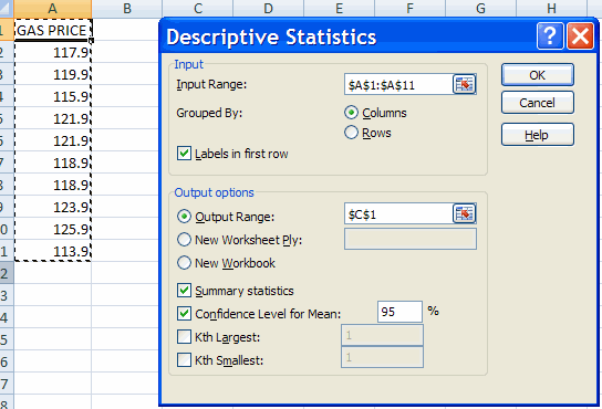
We consider gasoline price data (cents per gallon) in file gasolinepricedata.csv

• Read these data into Excel
• As detailed in Excel 2007: Descriptive Statistics
  - Access the Data Analysis Add-in on the Data Tab
  - Select descriptive statistics
  - In the Descriptive statistics dialog box provide the relevant information including  cehcking the confidence level box.
  

This yields

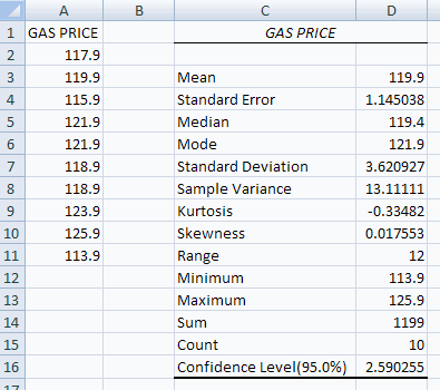
Then a 95% confidence interval for the population mean is

• The sample mean ("mean") plus or minus the "confidence level (95.0%)" reported by Excel
• i.e. mean ± confidence level (95.0%)
• Here this yields 119.90 ±- 2.59  =  (117.31, 122.49).

Interpretation: This means that with probability 0.95 the sample comes from a data generating process with population mean µ in the range 117.31 to 122.49.

To obtain confidence intervals at other levels of confidence, e.g. 90%, in Data | Analysis | Data Analysis | Descriptive Statistics change the confidence level for the mean from its default of 95% to e.g. 90%.

Note that since the sample is small here (n=10) this test requires the assumption that the data are normally distributed (see GENERAL COMMENTS at the top of this handout).
This assumption is impossible to test with only ten observations, but could be justified if (and I say if) experience with other larger samples of gasoline price data suggests that this is a resonable assumption.

FURTHER DETAILS ON CONFIDENCE INTERVALS FOR THE POPULATION MEAN µ

In general a symmetric confidence interval is of the form:
    estimate of the parameter of interest  ±  critical value × standard error.

For this particular problem, a 95% confidence interval for the population mean µ, when x is normal(µ,σ), is
   sample mean  ±  t(.025; n-1) × s/sqrt(n)
which can be calculated manually in Excel using:

• The critical value is that of a t-distribution with (n-1) degrees of freedom and area .95 in the center and .05 in the combined tails.
  
In Excel this can be calculated by the command =TINV(0.05,9) which yields a value 2.262157.
(Note that TINV reports results for two tails of the t distribution, not just one tail, so we use 2×.025 = 0.05).
Common textbook notation is to denote this t(.025;n-1) as there is area of .025 in the upper tail.
• The standard error is s / sqrt(n), the standard deviation (s) divided by the square root of the number of observations (n).
This is given in the second line of the descriptive statistics output as 1.145038.
This can also be calculated as the fifth line of the descriptive statistics output (3.620927) divided by the square root of 10.
• Combining we note that the critical value (2.262157) times the standard error (1.145038) yields 2.590255 (the confidence level).

THE CONFIDENCE( ) FUNCTION IS NOT USED.

In Formula Tab | Function Library | More Functions | Statistical is a function CONFIDENCE( ).
This computes the "Confidence level" when the standard deviation is known.
This is z(.025) × σ/sqrt(n)  for a 95% confidence interval.
We do not use this function because in economics examples σ is unknown and we instead use t(.025; n-1) × s/sqrt(n)

In summary, we do not use the CONFIDENCE( ) function as it leads to different results than Descriptive Statistics.

HYPOTHESIS TESTS FOR THE POPULATION MEAN µ

Hypothesis Tests for the Population Mean

Excel does not have an automatic command and output for hypothesis testing on the population mean.
Instead one needs to manually perform the hypothesis test using output from descriptive statistics.

We distinguish between one-sided and two-sided tests.
Let  µ0  denote the hypothesized value of µ.
Two-sided test:  H0: µ = µ0  against  Ha: µ not equal to µ0
One-sided test:  H0: µ <= µ0  against  Ha: µ > µ0
                     or:  H0: µ >= µ0  against  Ha: µ < µ0

We first find the value of a test statistic.
We then use either the p-value approach or the critical value approach to reject or not reject the null hypothesis that µ = µ0.

Test Statistic

A test statistic is often of the form:
    (estimated value - hypothesized value) / standard error
where the standard error gives the precision of the estimate.

For tests of H0: µ = µ0 we use the t-test statistic:
   t = (Xbar - µ0) / (s/sqrt(n)).

For the example here, to test H0: µ = 118 using the above data,
   t = (119.9 - 118) / 1.145038 = 1.659.

The t-statistic is t-distributed with (n-1) degrees of freedom under the null hypothesis that µ = µ0 and assuming that the individual observations are independent and identically distributed observations from a normal distribution with mean µ.

Note that since the sample is small here (n=10) this test requires the assumption that the data are normally distributed (see GENERAL COMMENTS at the top of this handout).
This assumption is impossible to test with only ten observations, but could be justified if (and I say if) experience with other larger samples of gasoline price data suggests that this is a reasonable assumption.

p-value approach

The p-value is the probability of just rejecting the null hypothesis.

In general we reject the null hypothesis at level α (alpha) if the p-value < α
and do not reject the null hypothesis at level α if the p-value >= α.
[A common choice of α is 0.05].

Let  T  be a t-distributed random variable and t be the calculated value of the test statistic.

• For test against Ha: µ not equal to µ0:  p-value = Pr(T <= -t or T >=  t).
• For test against Ha: µ > µ0:  p-value = Pr(T >=  t).
• For test against Ha: µ > µ0:  p-value = Pr(T <=  t) = 1 - Pr(T >  -t).

The p-value for hypothesis tests on the population mean µ is then obtained using the Excel commands:

• p-value for a 2-sided test:
pvalue = TDIST(1.659,9,2)  which yields a p-value of  0.131.
• p-value for a 1-sided test against Ha: µ > µ0:
  
p-value = TDIST(1.659,9,1) which yields a p-value of 0.066.
• p-value for a 1-sided test against Ha: µ < µ0:
  
p-value = 1 - TDIST(1.659,9,1) which yields a p-value of 1 - 0.066 = 0.934.

More generally we will have a different test statistic value than 1.659 and a different number of degrees of freedom than 9.

Critical values

Critical values are used to define a critical region.

If the calculated value of the test statistic falls in critical region then the null hypothesis is rejected. Otherwise it is not rejected.

Let  c  be the critical value of the test statistic and consider tests at level α (often α = .05).

• For test against Ha: µ not equal to µ0:  critical value is c such that Pr(T <= -c or T >=  c) = α.
• For test against Ha: µ > µ0:  critical value is c such that Pr(T  >=  c) = α.
• For test against Ha: µ < µ0:  critical value is c such that Pr(T <=  c) = α.

• For test against Ha: µ not equal to µ0:  t is such that  t <= -c or t >=  c.
• For test against Ha: µ > µ0:  t is such that t  >=  c.
• For test against Ha: µ < µ0:  t is such that  t <=  c.

The critical for hypothesis tests on the population mean µ is then obtained using the Excel commands:

• critical value for a 2-sided test:
critical value = TINV(.025,9)  which yields a critical value of 2.685.
• critical value for a 1-sided test
critical value = TINV(.05,9)  which yields a critical value of 2.262.

• For test against Ha: µ not equal to µ0:  t = 1.659  is not such that  t <= -2.685 or t >=  2.685.
• For test against Ha: µ > µ0:  t = 1.659 is not such that t  >=  2.262.
• For test against Ha: µ < µ0:  t = 1.659 is not such that t  <=  -2.262

Note that since the sample is small here (n=10) this test requires the assumption that the data are normally distributed (see GENERAL COMMENTS at the top of this handout).
This assumption is impossible to test with only ten observations, but could be justified if (and I say if) experience with other larger samples of gasoline price data suggests that this is a resonable assumption.

THE ZTEST( ) AND TTEST( ) FUNCTIONS ARE NOT USED.

In Formula Tab | Function Library | More Functions | Statistical is a function ZTEST( ).
This computes the t-test when the standard deviation is known.
It computes p-values using standard normal rather than t-distribution.
We do not use this function because in economics examples σ is unknown and we instead use the t-distribution.

In Formula Tab | Function Library | More Functions | Statistical is a function TTEST( ).
This performs a t-test of the difference im neans in two different samples.
This is a different t-test to the one presented above, where just a single sample is used.
The TEST( ) function does not do the t-test given above.

For further information on how to use Excel go to
  http://cameron.econ.ucdavis.edu/excel/excel.html